Differential equation in python
Sat 04 April 2020

Second orderdifferential equation(Photo credit: Wikipedia)
In python, differential equations can be numerically solved thanks to scipy [1]. Is usage is not as intuitive as I expected.
Simple equation
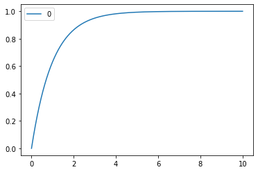
Let's start small. The first equation will be really simple:
The scipy ode module asks for equations written that way (\(\frac{\partial{f}}{\partial{t}}=fun(...)\))
def first_fun(y, t, a=-1, b=1):
    return a * y + b
This function takes as input:
- \(y\) : the value of \(f(t)\)
- \(t\) : the variable use by 'scipy ode'
- other parameters
Now let's define the variable t for which wee want a value:
import numpy as np


t = np.linspace(0, 100, 1000)
Now let's ask scipy for a solution:
from scipy.integrate import odeint


init_value = 0
solution = odeint(first_fun, init_value, t)
And let's plot it. As I am a lazy person, I'll let pandas plot it:
import pandas as pd


pd.DataFrame(solution, index=t).plot()
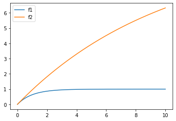
Multiple equations
Let's complicate things (a bit). The function can be multidimensional. This way, we can have multiple functions in our system of differential equations, either independent or not. In either way, we will build a function returning
and taking as input
def indep_fun(y, t, a1=-1, a2=.1, b1=1, b2=1):
    f1, f2 = y
    return [
        a1 * f1 + b1, # \frac{\partial{f1}}{\partial{t}}
        a2 * f2 + b2, # \frac{\partial{f2}}{\partial{t}}
    ]
And let's solve and plot it:
int_value = [0, 0] # [f1(0), f2(0)]
solution = odeint(first_fun, init_value, t)
pd.DataFrame(solution, index=t, columns=("f1", "f2")).plot()
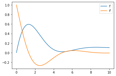
Second order differential equation
For that step, we need to take indirect routes. The basic principle is to use multiple equations, the second one being the derivative of the first one.
Let's say our equation is:
The input of our python function will be:
and the output:
Thus, the code is:
def second_order(y, t, a=-1, b=-1, c=.1):
    f, df = y
    return [
        df, # \partial{f}/\partial{t}
        a * df + b * f + c, # \partial^2 {f}/\partial{t}^2
    ]


init_value = [
    0, # f(0)
    1, # f'(0)
]
solution = odeint(first_fun, init_value, t)
pd.DataFrame(solution, index=t, columns=("f", "f'")).plot()
| [1] | scipy integrate module |
| [2] | notebook to generate graphs |